How Does Zorch Evaluate Constraints Without an Interpreter?

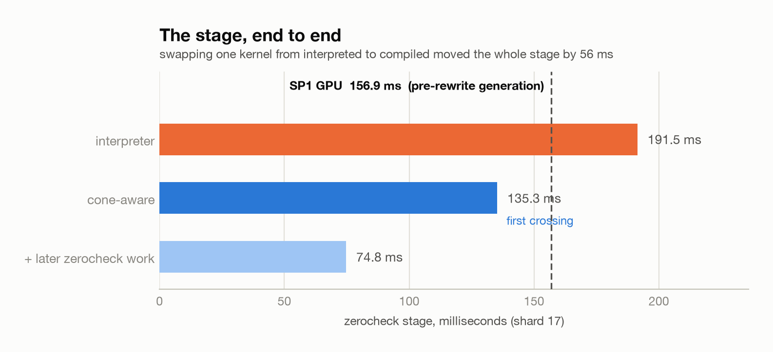
TL;DR Every major zkVM GPU prover today evaluates its AIR constraints with an interpreter: SP1 walks a bytecode tape, OpenVM walks monomial descriptors, ZisK walks an expression stream. There is a good reason. The alternative, compiling the constraint circuit into native GPU code, dies in the CUDA backend: a big chip unrolls into a ~400,000-line kernel that ptxas -O3 never finishes. Zorch (our ZK compiler stack: FRX, a fork of JAX, on top of our fork of XLA) takes the compile path anyway. The trick is not a bigger hammer; it is a schedule: you must cut the kernel to compile it, and you can only cut where few values are live, so emit the circuit in a minimum-live order first. Cone-aware scheduling plus outlining brought compile time 613 s → 19.5 s, made the kernel 2.34× faster than the interpreter (1,489 → 635 µs), moved the zerocheck stage 191.5 → 135.3 ms, under the 156.9 ms of SP1's GPU prover at the time, and keccak, which previously did not compile at all, compiles.

0. Scope and terminology

Zorch: our ZK proving stack built around a compiler. Constraints and provers are written against FRX (our fork of JAX, adding finite-field types and ops) and compiled by our fork of XLA (adding ZK codegen). Throughout this article, FRX and XLA refer to these forks.
Comparison target: SP1's GPU prover (succinctlabs/sp1). One caveat up front: SP1's zerocheck prover is not one design. Our benchmarks compare against the generation that existed through early 2026 (a bytecode interpreter); upstream replaced it on 2026-06-09 with a DAG-native prover (#2795), still interpreted, and remarkably convergent with this article's ideas (§2.1).
"Cone": standard circuit-theory vocabulary (logic cone in synthesis, cone of influence in model checking): everything reachable backwards from an output node. Here, the backward slice of one constraint.

1. Background: why constraint evaluation

1.1 It is the most expensive stage

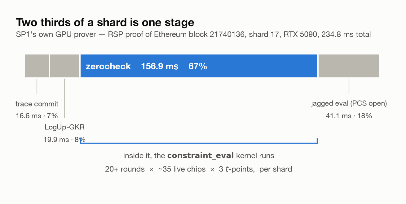
Profile SP1's own GPU prover over a real workload, shard 17 of an RSP proof of Ethereum mainnet block 21740136 (RTX 5090, warm, byte-matched), and one stage dominates:

Stage	SP1 GPU	share
trace commit	16.6 ms	7%
LogUp-GKR	19.9 ms	8%
zerocheck	156.9 ms	67%
jagged eval (PCS open)	41.1 ms	18%
full shard	234.8 ms

(Measurement setup and the current comparison table live in sp1-zorch's dev docs.)

Two thirds of the wall clock is one stage. Nothing else matters until this does.

1.2 What zerocheck computes

Zerocheck proves "every AIR constraint is zero on every real row" via sumcheck:

\sum_{\vec x \in \{0,1\}^{n}} \widetilde{\mathsf{eq}}(\vec\zeta, \vec x)\; C_\alpha\big(\mathrm{trace}(\vec x)\big) = 0

Unpacking the symbols:

$\mathrm{trace}(\vec x) \in \mathbb{F}^{c}$ is the column-value vector of the row indexed by $\vec x$ ( $n$ bits). The trace is a $[2^n \times c]$ matrix; treating the row index as a hypercube point gives its multilinear extension, which is defined off the hypercube too, and that matters in a moment.
$C_k : \mathbb{F}^{c} \to \mathbb{F}$ is one AIR constraint: a low-degree polynomial over column values, required to vanish on real rows. The verifier's randomness $\alpha$ batches $K$ of them into one: $C_\alpha(\vec v) = \sum_{k} \alpha_k C_k(\vec v)$ (Transition constraints take the current and the next row; we write one vector to keep notation light.)
$\vec\zeta$ is a random evaluation point chosen by the verifier (in the real pipeline it is handed down by LogUp-GKR). Without the $\widetilde{\mathsf{eq}}(\vec\zeta,\cdot)$ weighting, nonzero rows could cancel and the bare sum could still be zero; under random weighting, "the sum is zero" forces "zero on every row" with overwhelming probability (Schwartz–Zippel).

Sumcheck eliminates one row variable per round. Within a round, split the current trace buffer by the variable being eliminated:

p_0 = \mathrm{trace}\big|_{x_i=0}, \qquad p_1 = \mathrm{trace}\big|_{x_i=1}, \qquad \Delta = p_1 - p_0

The trace is multilinear, hence linear, in $x_i$ , so the trace at point $t$ is just $p_0 + t\cdot\Delta$ (this is where "defined off the hypercube" pays off). The round polynomial has degree 4, but Gruen's trick means only $t \in \{0,2,4\}$ need be evaluated. So the hot loop of one round is:

y_t = \sum_{\text{rows}} \underbrace{C_\alpha\big(p_0[\text{row}] + t\cdot\Delta[\text{row}]\big)}_{\texttt{constraint\_eval}} \cdot \mathrm{eq}[\text{row}]

( $p_0[\text{row}], \Delta[\text{row}]$ are that row's column vectors; $\mathrm{eq}[\text{row}]$ is a precomputed weight table.) The math ends here. Everything from now on is systems.

1.3 The hot core: `constraint_eval`

constraint_eval is the circuit that evaluates $C_\alpha$ for one row. The eq-weighted reduction and Gruen assembly are separate ops; this circuit is a pure row-parallel map, one thread runs the whole circuit for one row:

   row 0 ─┐
   row 1 ─┤   ┌──────────────────────────────────────────┐
   row 2 ─┤──▶│  C_0  C_1  C_2  ...  C_{K-1}             │──▶ out[row]
     ...  ┤   │   └────┴────┴──────── α-fold ─────┘      │
   row N ─┘   └──────────────────────────────────────────┘
          how to turn this per-row circuit into a kernel = this whole article

The circuit is not small:

	Global (SP1 CPU chip)	KeccakPermute (SP1 precompile)
constraints $K$	216	~2,900
trace columns	hundreds	2,640
serialized	3,583 field ops	~50,000 instructions

And the call count multiplies: every round × every live chip × three $t$ -points (20+ rounds, ~35 main chips). Swapping just this kernel from interpreted to compiled moved the whole zerocheck stage 191.5 → 135.3 ms, and a large share of the stage lives here.

This is not an SP1-specific problem. Any AIR-based zkVM (SP1, OpenVM, ZisK, RISC Zero) has this loop in some form. (Lookup-centric designs like Jolt are the exception.)

1.4 Where the circuit comes from

Two lines of background for readers who don't know the ML-compiler world. JAX is a numerical framework that traces Python programs into StableHLO graphs; XLA is the compiler that turns those graphs into CPU/GPU kernels. Our FRX is a fork of JAX (field types and ops); our XLA fork adds ZK codegen.

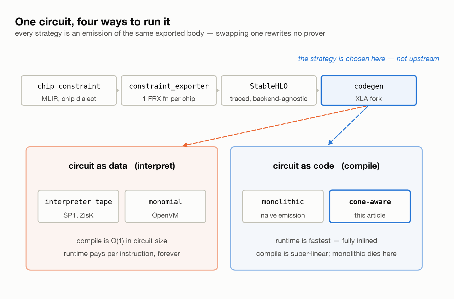
In Zorch, a constraint's journey is:

riscv-witness                      export                       XLA (our fork)
┌─────────────────────┐   ┌───────────────────────┐   ┌──────────────────────────┐
│ chip constraint     │──▶│ constraint_exporter   │──▶│ zorch.constraint_eval    │
│ (MLIR, chip dialect)│   │ → 1 FRX fn per chip   │   │ marker → GPU/CPU codegen │
└─────────────────────┘   └──────────────────────-┘   └──────────────────────────┘
                              └─ traced to StableHLO ──┘

Concretely, SP1's Add chip is defined like this:

// SP1 Add chip constraints — 15 constraints matching SP1 AddChip::eval() order.
chip.constraint_fn @sp1_add_constraints(%row: !chip.row<@sp1_add_schema>) -> tensor<15x!F> {
  %is_real = chip.get_col %row, "is_real"          : ... -> !F
  %b       = chip.get_col %row, "op_b_prev_value"  : ... -> tensor<4x!F>
  %c       = chip.get_col %row, "op_c_prev_value"  : ... -> tensor<4x!F>
  %value   = chip.get_col %row, "value"            : ... -> tensor<4x!F>

  // c0: is_real ∈ {0, 1}
  %c0 = func.call @assert_bool(%is_real) : (!F) -> !F
  // c2..c5: carry chain — carry_i = (b[i] + c[i] + carry_{i-1} - value[i]) · inv(2¹⁶)
  %c2_c5 = func.call @assert_add_carry_4(%b, %c, %value, %is_real) : ... -> tensor<4x!F>
  ...
  %packed = chip.pack_constraints(%c0, %c1, %c2_c5, ...) : ... -> tensor<15x!F>
  chip.return %packed : tensor<15x!F>
}

The exporter inlines every helper, unrolls every loop, and emits one batched [N, cols] → [N, K] FRX function per chip. Its shape (a sketch, since the real output is exactly this kind of fnp code; transition constraints take a second arg1 for the next row):

import frx.numpy as fnp

def sp1_add_constraints(arg0):              # arg0: [N, cols] — a batch of rows
    is_real = arg0[:, 0:1]                  # column indices fixed by the schema
    b0      = arg0[:, 12:13]
    ...
    v0 = is_real * is_real - is_real        # c0: assert_bool, inlined
    v1 = (b0 + c0_ + carry_prev - value0) * inv_2_16   # carry chain, unrolled per limb
    ...
    return fnp.concatenate([v0, v1, ...], axis=1)      # [N, 15]

The Add chip ends there. A bignum precompile unrolls its limb loops into tens of thousands of lines of the same shape, which is the keccak ~50,000 in §1.3's table.

Two properties to plant here. First, the chip MLIR is tied to no proof system and no backend: it is not lowered directly to anything; it is exported to FRX, traced to StableHLO, and only at the final codegen stage of the XLA fork does the evaluation strategy get chosen. Second, that means one exported body is the single common input to every strategy this article discusses: monolithic, interpreter, cone, monomial are all swappable emissions of the same circuit.

So from the compiler's seat, the input is: a branch-free, pure field-arithmetic DAG of thousands to tens of thousands of nodes. No branches is a blessing (the schedule is completely free); the size is the curse.

1.5 Circuit as code, or circuit as data

There are two ways to turn that DAG into a GPU kernel, and each hits a wall:

	circuit as code (compile)	circuit as data (interpret)
runtime	fastest, fully inlined, zero interpretation cost	per-instruction interpretation cost, and not just decode (§2.4)
compile	super-linear in circuit size, big chips never finish	O(1), kernel size independent of the circuit
big chips	✗ (ptxas: 30 min–2 h, OOM)	✓

The main body of this article answers two questions:

How do you get compiled-code speed and still have compilation finish? Cut the kernel into pieces, but cutting anywhere makes things worse, measurably (§3.2).
Per-constraint emission duplicates shared work. Cones overlap: one Poseidon2 permutation feeds 163 constraints. Deduplicate, and registers become the next problem (§3.5).

Calibrating the three time scales in this article.

time	scale	why it matters
kernel execution	µs	short once, but runs dozens of times per stage (chips × 3 $t$ -points × rounds). Changing this one kernel 1,489 → 635 µs moved the stage by 56 ms
zerocheck stage	ms	one shard proves in ~235 ms and a block is dozens of shards, so stage milliseconds are proving throughput
kernel compile	s–hours	rules the dev loop and cold start. 613 s = "10 minutes per circuit tweak"; keccak's 1–2 h + OOM = "this chip cannot be proven on GPU at all"

2. State of the art: everyone interprets

Before our answer, the industry's. Every major zkVM GPU prover evaluates constraints with an interpreter: the circuit lives in device memory as data, and a fixed kernel walks it. Three data points, with code:

2.1 SP1: a bytecode tape (two generations)

The generation we benchmarked against (through early 2026; zerocheck_eval.cu @ 98ce1c3):

crates/air (sp1-gpu)                                  zerocheck_eval.cu
┌───────────────────────────┐  regalloc  ┌───────────┐  ┌───────────────────────────┐
│ SymbolicProverFolder      │───────────▶│Instruction│─▶│ for (i in program)        │
│  traces constraints into  │ optimizer  │16 tape    │  │   switch (instr.opcode) { │
│  an Instruction32 list    │ (liveness+ │+ consts   │  │     case FAddVV: ...      │
└───────────────────────────┘ first-fit) └───────────┘  │     case EMulEE: ... }    │
                                                        │ K expr_f[MEMORY_SIZE]     │
                                                        └───────────────────────────┘

Constraints are traced symbolically into a three-address instruction list; a host-side liveness-based register allocator (optimizer.rs: free at last use, first-fit reuse) compresses it into an Instruction16 tape plus a peak register count, which selects a kernel variant with scratch array K expr_f[MEMORY_SIZE], MEMORY_SIZE ∈ {32 … 1024}. The kernel interprets the tape per row through a switch over ~76 opcodes.

The current generation: on 2026-06-09 upstream deleted all of the above and landed the DAG-native prover (#2795; ir/chunker.rs, sequential.cu): constraints are built into one ConstraintDag with explicit cross-constraint sharing, then packed into chunks by a greedy first-fit-decreasing chunker under a register-pressure budget (leafset ≤ 64 → downstream max_reg ≲ 128 → a MAX_REGS ∈ {32…1024} kernel tier). Execution is still bytecode interpretation (switch (instr.opcode) over BcOp).

Note the convergence: shared-DAG CSE and peak-live-as-a-first-class-budget are exactly the two pillars of §3. Two teams arrived at the same structure from opposite sides, which is good evidence this is the shape of the problem, not an implementation quirk. Note also what SP1's pipeline is: trace → IR → register allocation → bytecode. That is a small bespoke compiler, targeting bytecode instead of native code. Hold that thought for §5.

Benchmark caveat: the SP1 GPU numbers in this article (156.9 ms etc.) measure the pre-rewrite generation. Comparing against current main needs re-measurement.

2.2 OpenVM: monomials as data

OpenVM's CUDA backend (stark-backend v2) flattens constraints into monomial form and stores them as device buffers: packed variable descriptors and per-monomial headers (monomial.cuh):

// Packed variable: 4 bytes
// Bits 0-3: entry_type / 4-11: part_index / 12-15: offset / 16-31: column_index
struct PackedVar { uint32_t data; ... };

// Monomial metadata
struct MonomialHeader { uint32_t var_offset; uint32_t term_offset;
                        uint16_t num_vars;   uint16_t num_terms; };

The monomial-MLE kernels (batch_mle_monomial.cu) walk these descriptors: eval_variable decodes a packed variable and loads its column, and per-monomial loops multiply the variables and fold the batching coefficients. Different encoding, same species: a fixed kernel walking the circuit as data.

2.3 ZisK: an expression stream

ZisK proves with Polygon's pil2-proofman; its GPU expression evaluator (expressions_gpu.cu @ v0.18.0) is the most literal interpreter of the three: an ops stream compiled from PIL at setup time, dispatched op by op:

switch (op) {
    case 0: C[threadIdx.x] = A + B; return;
    case 1: C[threadIdx.x] = A - B; return;
    case 2: C[threadIdx.x] = A * B; return;
    case 3: C[threadIdx.x] = B - A; return;
}

So the pattern holds across SP1, OpenVM, and ZisK. It is a rational pattern: the kernel is O(1) in circuit size, so the compile wall of §1.5 simply never appears. The question is what it costs.

2.4 What interpretation costs: it is not just decode overhead

Four layers, from shallow to deep:

Fetch + decode + branch. Every instruction reads the tape and takes a switch branch, a fixed tax that is large next to a field add (a few native instructions). (Threads in a warp mostly run the same program, so opcode divergence is minor; the tax is the dispatch itself and the serialization around it.)
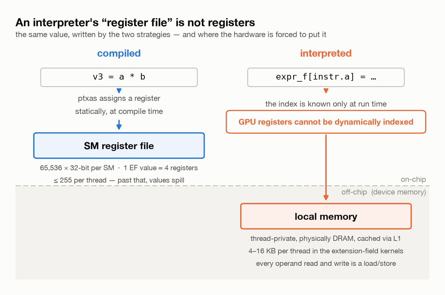
The register file that isn't. ★ This one deserves a close look. The interpreted program's "registers" are an array indexed at runtime: expr_f[instr.a] in SP1's old kernel, regs[instr.out] in the new one. GPU hardware registers cannot be dynamically indexed, so the compiler is forced to place these arrays in local memory, thread-private storage that physically lives in device memory, cached through L1. This is structural, not an implementation detail: every operand read and write becomes a load/store. SP1's own source says it plainly: the DAG-native chunker keeps chunks small so the per-thread array stays inside "the L1-cached local-memory window" (chunker.rs), and in the extension-field kernels that array alone is 4–16 KB per thread. So when SP1's new prover budgets "max_reg ≲ 128", those are slots in a local-memory array, not physical registers. Compiled straight-line code is the only way interpreted values become register-resident: ptxas assigns actual registers statically. (That is also why §3.5's register arithmetic is about the real 64K-per-SM register file.)
Lost ILP. GPU cores are in-order; instruction-level parallelism comes from compile-time scheduling. In compiled code, ptxas interleaves independent field ops to cover load latency. In an interpreter, every operation sits behind the same fetch → branch → execute dependency chain, so neither the hardware nor the compiler can see that two adjacent tape instructions are independent.
Lost cross-op optimization. Compiled neighbors get folded: constants propagate, common subexpressions stay in registers, multiplication internals can stay in intermediate form across ops. An interpreter's opcode routines are generic: every op is a complete, self-contained computation.

There is one honest counterpoint: an interpreter's code is tiny, so it never worries about instruction-cache pressure, and a 450,000-line compiled kernel pays for instruction fetch too. But the sum is lopsided: on the same circuit, our interpreter measured 1,489 µs/exec vs 635 µs/exec compiled, 2.34× (§4).

We know the interpreter arm well because we built one too: same design, a tape interpreted by an scf.for loop. It carried us past the compile wall (CPU byte-match went from 1 h+ timeouts to ~30 s) and it was the thing the cone path eventually had to beat.

3. The compiler path: making the circuit compile

Rewriting the problem from the compiler's seat, there are three sub-problems:

Size: emitted as code, the circuit is so large the backend (ptxas/LLVM) dies super-linearly.
Duplication: emitted per constraint, overlapping subgraphs are recomputed.
Pressure: deduplicate, and values live long enough to exhaust registers.

They pull against each other: fixing one worsens another. This section walks the chain in the order the design actually resolved it.

3.1 The unit of cutting: cones

The body the emitter receives has a fully unrolled alpha-fold chain at its root:

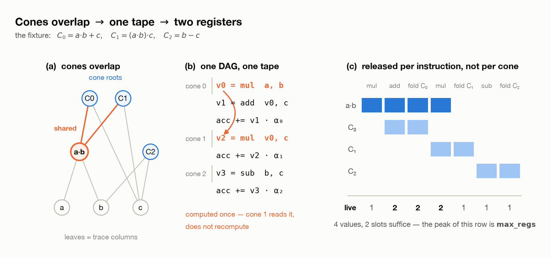
\mathrm{acc}_0 = C_0\alpha_0,\quad \mathrm{acc}_k = \mathrm{acc}_{k-1} + C_k\alpha_k

Reading the chain backwards at HLO level, the non- $\alpha$ operand of each multiply is a $C_k$ ; the backward slice from that node is a cone, everything constraint $k$ actually depends on.

        C_0        C_1        C_2         ← cone roots (one per constraint)
         ▲          ▲          ▲
         │    ╱─────┴──╲       │
         └───●  shared  ●──────┘          ← cones overlap!
            ╱     ▲      ╲
          col0   col1   col2              ← leaves = trace columns / constants

Why this unit? Because it is a boundary the circuit already had: the moment a constraint folds into the accumulator, most of its intermediates die. It is not an arbitrary line: it is where values naturally end, and §3.6 depends on exactly that.

Recognition is conservative: any unrecognized pattern anywhere makes the planner return nullopt and fall back to the original monolithic body. The contract is one line: correct-but-slow, never a miscompile. The price is real too: on wide chips that fallback is ~20× slower, so recognition coverage is itself a performance problem.

3.2 Outlining, and why cutting anywhere loses

The size fix itself is obvious: cut the function. Slice the straight-line kernel into contiguous regions, hoist each into a device function, leave calls behind. The backend then only ever sees small pieces:

   before — one function                     after
   ┌───────────────────────┐                ┌──── entry ─────────────┐
   │ v0 = mul …            │                │ … = call region_0(…)   │──▶ ┌─ region_0 ─┐
   │ v1 = add …            │                │ … = call region_1(…)   │    │ v0 = mul … │
   │    (450k lines)       │      ──▶       │                        │    │ return …   │
   └───────────────────────┘                └────────────────────────┘    └────────────┘
      ptxas never finishes                      each piece is tractable

(Note this is not splitting the kernel: the functions stay inside one kernel, operands travel in registers, and there is no HBM round-trip.)

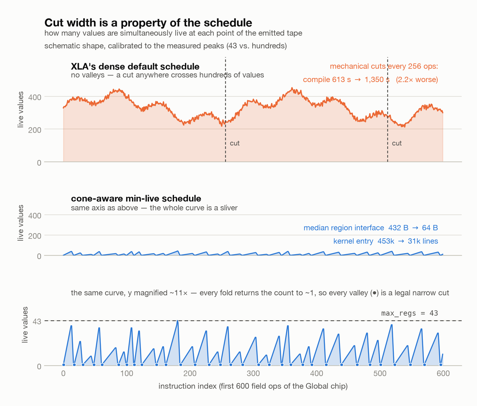
We tried the obvious version: cut the original XLA body mechanically every 256 ops. Result:

\text{compile } 613\,\mathrm{s} \;\longrightarrow\; 1{,}350\,\mathrm{s} \qquad (2.2\times\ \text{worse})

The hidden cost of a cut is the set of live values crossing it: everything made before the cut and still needed after must be returned by the region and held by the entry. In XLA's dense schedule, every cut crossed hundreds of values; each chunk returned ~256 extension-field values, forcing a memory ABI and spills. Shrinking the chunk didn't help: the boundary stayed saturated.

This is where the perspective flips, the pivot of the whole design:

❌ "choose better cut points"        →  a dense schedule has no good cut points
✅ "emit in an order that creates
    good cut points"                 →  fix the schedule first

Cut width is a property of the schedule. The order you emit instructions decides how many values are live across any given point. Building that order is §3.4 and §3.5; first, one more thing the emitter must understand about its input.

3.3 Lanes: shape operations for free

The exported body is not a scalar circuit: it is a tensor program full of slice / broadcast / concatenate / reverse / transpose. Emitting those as code would be absurd; instead the emitter tracks, for every element of every intermediate tensor, where that value comes from, a lane (a register, a trace column, a constant, and so on).

Then every shape-only operation becomes index algebra on lane vectors, zero instructions:

HLO	lane treatment	instructions
reshape / bitcast / copy	pass through	0
broadcast / slice / concatenate / reverse / transpose	index permutation	0
reduce (add)	fold lane group into an add chain	chain per group
elementwise add/sub/mul/negate	one instruction per lane	lanes
anything else	unrecognized	→ monolithic fallback

A real fixture (an EC-shaped chip, 4 columns, 4 constraints): the HLO body contains 8 shape ops and 6 elementwise ops, and compiles to exactly 6 field instructions. The 8 shape ops cost nothing.

Why it matters: keccak's constraints are full of per-row bit-order reverse; bignum chips use band-sum transpose and bit-pair concatenate. If the lane model doesn't absorb those, the whole chip falls back to monolithic (~20×), and this is half of what saved keccak (§4). And it is the bridge that makes §1.4's claim free: we accept an implementation-independent tensor IR and still emit scalar-optimal code. (One designed limit: permutations that touch the row axis always fall back, since rows are the parallel axis, not lanes.)

3.4 One DAG, registers that outlive cones

Now duplication. Cones overlap: if $C_0$ and $C_1$ both use $a\cdot b$ , expanding each cone independently doubles the multiply; with Poseidon2's 163-cone shared permutation it 163×'s it.

The fix is to serialize all cones into one tape under two rules. A real test fixture, columns $a, b, c$ , three constraints:

C_0 = a\cdot b + c, \qquad C_1 = (a\cdot b)\cdot c, \qquad C_2 = b - c

tape                                    notes
──────────────────────────────────────────────────────────────
cone 0 ┌ v0 = mul  a, b                 a·b, shared. computed HERE, once
       │ v1 = add  v0, c                C0
       └ acc += v1 · α[0]               cone 0 ends → folds immediately
cone 1 ┌ v2 = mul  v0, c                C1  ★ v0 is NOT recomputed
       └ acc += v2 · α[1]
cone 2 ┌ v3 = sub  b, c                 C2
       └ acc += v3 · α[2]
──────────────────────────────────────────────────────────────
4 field ops (mul, add, mul, sub)

Rule ①: walk a DAG, not per-cone trees. In the original HLO, a·b is one node that both $C_0$ and $C_1$ point at. Serialization emits one value per node, in the earliest cone that needs it.
Rule ②: the register file survives across cone boundaries. Cone 0 ending does not clear v0's slot; cone 1 reads it directly. ① alone is useless without this, since clearing registers at each cone means you recompute regardless of sharing.

Duplication solved: every shared value is computed exactly once. But look at what rule ② does: it keeps values alive longer. That is the next problem.

3.5 Pressure: real registers this time

Why "live value count" is destiny on a GPU

On a GPU, scalar values live in registers, and registers are a physically shared resource:

One SM has a register file of 65,536 32-bit registers (recent architectures).
One thread can use at most 255; beyond that, values spill to local memory.
Resident warps per SM ≈ $65{,}536 / (\text{regs/thread} \times 32)$ : the more registers per thread, the fewer warps are resident, and the worse the GPU hides memory latency.

Our values are heavier still: an extension-field element is four 32-bit registers. So "peak live EF values × 4" is the per-thread register demand, and that number directly sets (a) resident warps, (b) spill, (c) whether the backend's register allocator terminates at all.

(Contrast with §2.4: these are physical registers. The compiled path is the only one where this arithmetic applies, since interpreted values never get here.)

You cannot keep everything alive

Push cross-cone reuse to the limit and chips answer differently:

   Global :  ▁▂▃▄▃▂▃▄▃▂▁ …               peak 43     ← fine
   keccak :  ███████████████████ …       peak 2,300  ← disaster

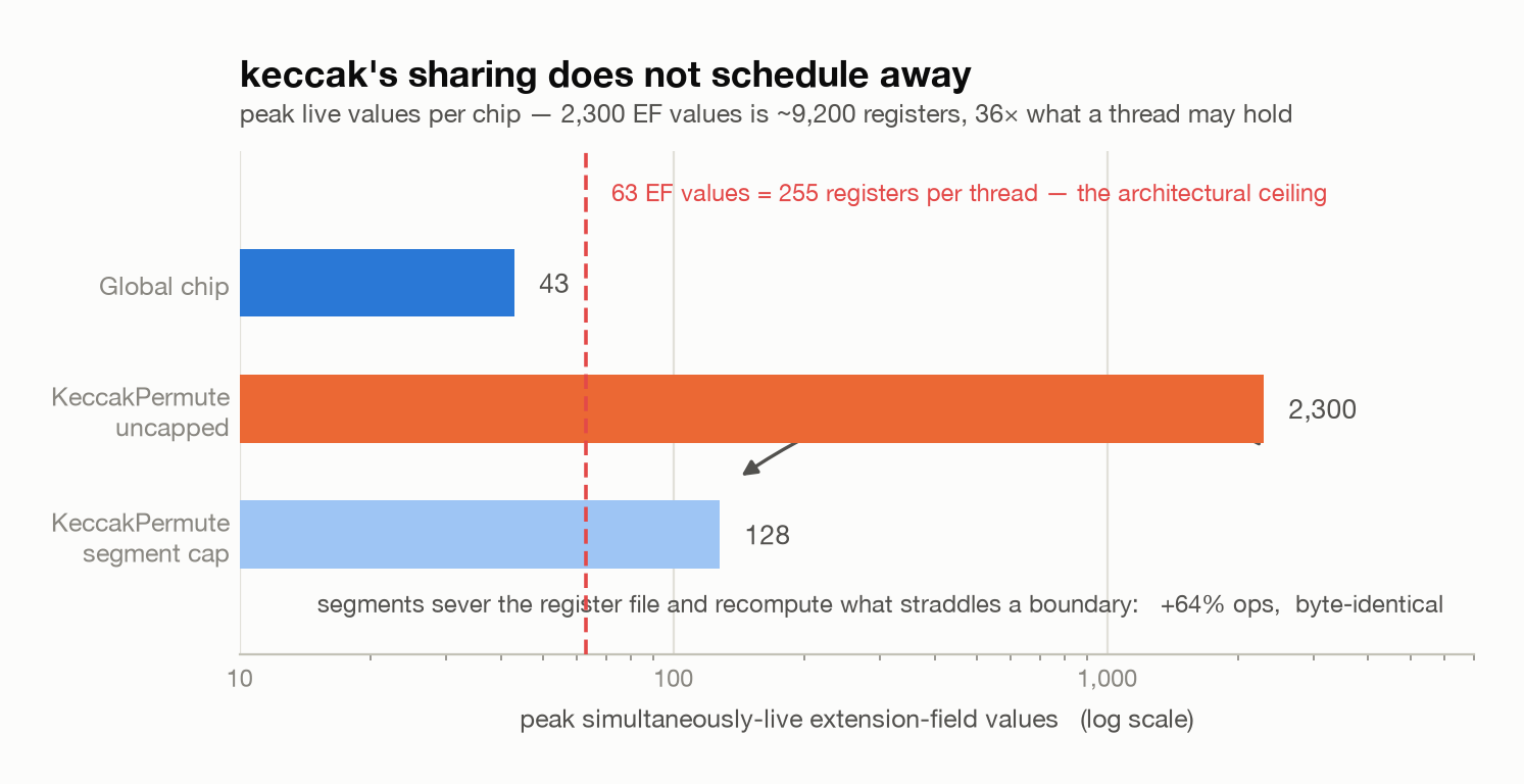
keccak's sharing is wide: peak 2,300 live EF values ≈ 9,200 registers, 36× the architectural limit. Everything spills, and before that, LLVM's register allocator effectively never terminates on the interference graph.

Measure the peak: the min-live-set schedule

So the scheduler computes exact liveness while emitting: a value is born in the earliest cone that needs it, and its slot is released immediately after its last use, per instruction, not per cone. The live ranges of §3.4's example:

value	①`mul`	②`add`	③fold C₀	④`mul`	⑤fold C₁	⑥`sub`	⑦fold C₂
`ab`	█	█	█	█
`C0`		█	█
`C1`				█	█
`C2`						█	█
live	1	2	2	2	1	1	1

ab alone lives across cones (last used at ④); everything else dies into the fold that consumes it. Four values, but two slots suffice: slot 1 is reused three times. The maximum of the live row is the tape's max_regs:

\texttt{max\_regs} = \max_{\text{instruction}}\big(\#\text{values live at that point}\big)

Real scale: the Global chip is 3,583 field ops with max_regs = 43: of 3,583 values, at most 43 are ever simultaneously alive. Per-instruction release is what makes this minimal; releasing at cone boundaries would inflate the peak.

When even the schedule isn't enough: the pressure cap

keccak's 2,300 does not schedule away: the sharing really is that wide. One knob remains: give back some reuse. Group cones into segments with a hard rule, peak live within a segment ≤ 128 (segment length found by greedy doubling and bisect), and deliberately sever the register file at segment boundaries. Shared values that straddle a boundary are recomputed by the next segment:

\text{live } 2{,}300 \;\longrightarrow\; 128, \qquad \text{ops } +64\%

That is keccak measured: 38,283 field ops at peak 128. Recomputing 64% hurts, but the trade is "doesn't compile + spills everything" vs "+64% arithmetic". The accumulation order is untouched, so results stay byte-identical; chips with low peaks (Global) never trigger the cap.

Rule ② of §3.4 and this cap point in exactly opposite directions. Reuse and pressure are two faces of one coin, and the cap is the explicit knob between them: the compiler doesn't know "the answer", it turns the trade-off into a measurable parameter.

3.6 The cut is the function signature

Back to outlining, now with the schedule in hand.

Cut at any point and the values live across it become the outlined function's interface: the region must return them, the entry must hold them, and if there are too many they degrade to an out-pointer (memory) ABI. Compare two cut candidates on §3.4's tape:

   tape                              candidate A     candidate B
   ────────────────────────────────────────────────────────────
   v0 = mul  a, b
   v1 = add  v0, c
   acc += v1 · α₀                    ─── A ───
   v2 = mul  v0, c
   acc += v2 · α₁                                    ─── B ───
   v3 = sub  b, c
   acc += v3 · α₂
   ────────────────────────────────────────────────────────────
   values crossing                   v0, acc          acc

A: v0 is still alive (the very next mul uses it) → two values cross.
B: v0 is past its last use → only the accumulator crosses.

Now re-read §3.5's live row 1 2 2 2 1 1 1: it was secretly the table of "how many values cross if you cut here." Cut width is live count:

\boxed{\text{cut-width} \;\le\; \texttt{max\_regs}}

The min-live-set schedule flattened that whole row, so every cut is already narrow, and the outliner just picks the narrowest. This is precisely what generic chunking lacked: in XLA's dense schedule that row read in the hundreds everywhere.

The algorithm is a sliding window:

   ① from the current position, view [ +min_chunk , +region_cap ] as a window
   ② choose the cut candidate inside it with the fewest crossing values
      (ties → latest position, to keep pieces long)
   ③ cut there, restart ① from the cut

The outliner knows nothing about cones. It only minimizes crossings, and lands on cone-segment boundaries anyway, because that is where values naturally die (§3.1), and past a segment boundary the next segment recomputes its own shared values (§3.5), so essentially only the accumulator crosses.

Measured: median region return interface 432 B → 64 B; kernel entry 453k → 31k lines.

3.7 Thresholds, and the last ptxas wall

Piece size has walls on both sides: too small and call-boundary costs (marshalling, lost scheduling freedom) eat the gains; too large and §3.2's compile wall returns. Three knobs:

knob	value	meaning
min chunk	16 ops	shorter pieces aren't worth a call, so they stay inline
region cap	4,096 / 1,024	upper bound on one outlined function (a window size, not a stride)
cone floor	3,400 ops	circuits below this never take the cone path, they stay monolithic

Two decisions here are the compiler being honest with itself:

The floor: small circuits should stay monolithic. Monolithic compilation, when it finishes, is the fastest runtime: fully inlined, zero call boundaries, maximal ptxas freedom. So chips below the floor are deliberately left monolithic. The cone path does not beat monolithic; it goes where monolithic cannot. At that size its real competitor was the interpreter, and that it beat, 2.34×.

The adaptive cap: the criterion is execution, not compilation. Chips whose body exceeds 20,000 ops (keccak ~46k) drop the region cap 4,096 → 1,024. At 4,096 the regions spill ~23 KB/thread; multiply by occupancy, add the shard's resident buffers, and the kernel fails at launch: it compiled, but doesn't run. At 1,024 spill falls to ~7 KB and launch fits. Light chips keep 4,096, with no reason to fragment their call structure.

And then ptxas un-does it. At keccak scale (PTX 30–260 MB), ptxas -O3 re-inlines every outlined function: PTX has no no-inline directive, so whole-program optimization merges the regions back into the entry and register allocation explodes (1–2 h, 50 GB RSS, OOM). The fix is physical separation of compile units: above 16 MB of PTX, switch to relocatable compilation (ptxas -c + nvlink). Each region becomes its own -O3 unit; re-inlining is structurally impossible. Ordinary kernels keep the single-pass path, since where inlining wins, nothing should stop it.

4. Results

Global chip (block 21740136, shard 17, RTX 5090)

Isolated benchmark, one circuit, three strategies:

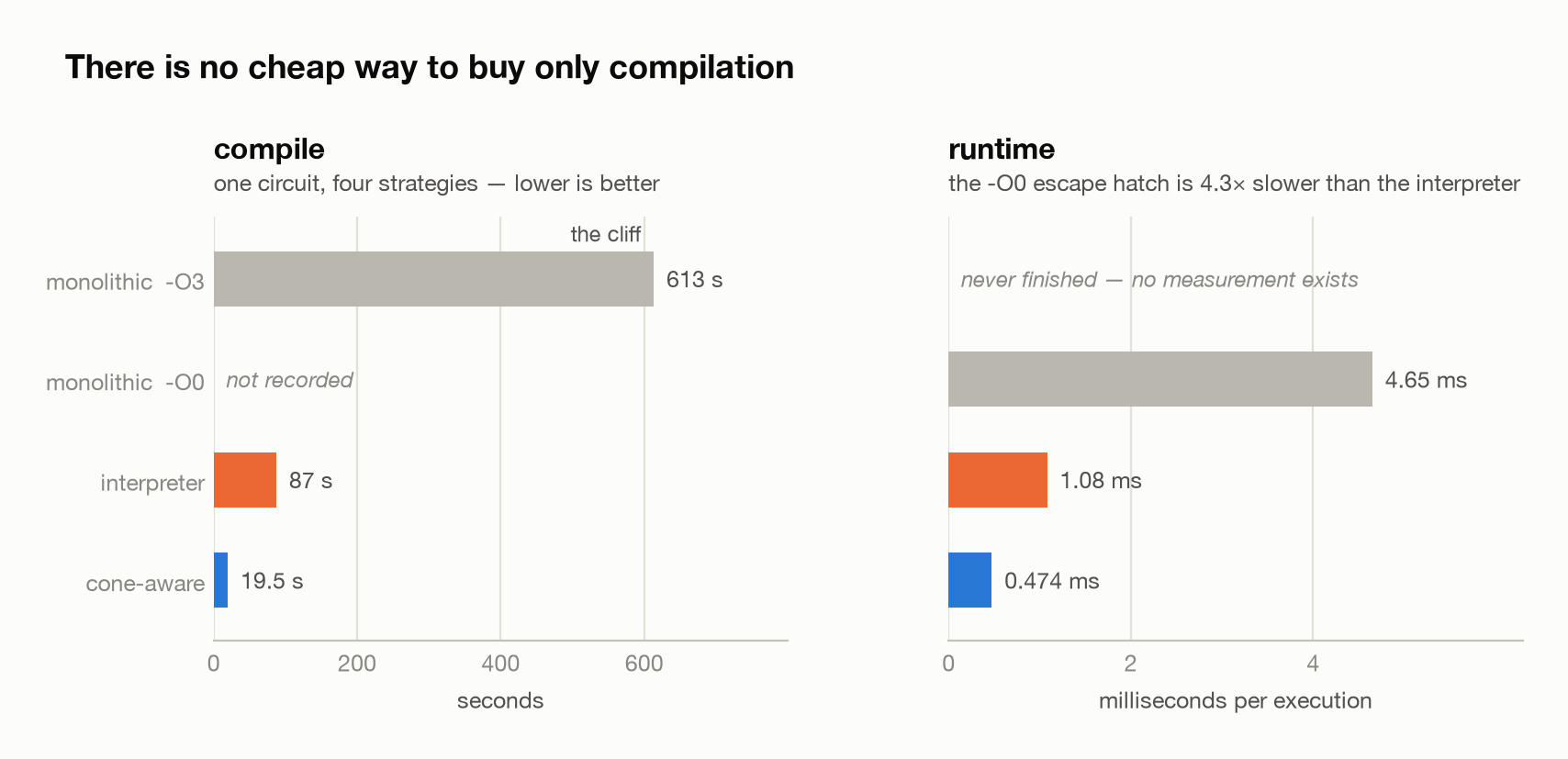
	monolithic	interpreter	cone-aware
compile	613 s (cliff)	~87 s	19.5 s
runtime	n/a¹	1.08 ms	0.474 ms
outlined functions	n/a	n/a	71
function arity	(256)	n/a	max 37 / avg 26

¹ -O3 never finished, so no measurement exists. The -O0 escape hatch ran at 4.65 ms, 4.3× slower than the interpreter. There is no cheap way to buy only compilation.

End-to-end:

	interpreter	cone-aware
`constraint_eval` kernel	1,489 µs/exec	635 µs/exec (2.34×)
zerocheck stage	191.5 ms	135.3 ms
SP1 GPU, same stage	156.9 ms	first crossing

(The SP1 figure is the pre-rewrite generation, see §2.1's caveat.)

CPU moves the same way: compile 138 s → 1.62 s, runtime 1.25 → 0.58 s/exec.

KeccakPermute: from impossible to running

Precompile chips are a different fight: previously they did not compile at all (ptxas 1–2 h then OOM). With the pressure cap (§3.5) plus adaptive cap and relocatable compilation (§3.7) together:

The KeccakPermute shard's zerocheck compiles and runs on GPU, byte-identical to SP1.

All strategies are byte-identical

Field addition and multiplication are exact, so reassociation and distribution produce the same element, and the alpha-fold order is never touched. Monolithic, interpreter, and cone emit bit-identical proofs, so the choice is purely about performance, and every number above was measured behind a byte-match gate against the SP1 reference.

The numbers in this article are from the cone work itself. Zerocheck has since accumulated further optimizations (shrink-prefix shared round buffer, in-kernel folds, and others); the same shard currently measures 74.8 ms, 0.48× of SP1 GPU, in the up-to-date table.

5. Could SP1, OpenVM, or ZisK just do the same?

Fair question, and the honest answer is: nothing stops them in principle. But walk through what "the same" requires.

Emitting native code is the easy part. Anyone can print CUDA C++ from a constraint AST. Naive emission is exactly the monolithic arm of §4: on a real chip the backend dies (613 s cliff; keccak hours-then-OOM). This wall is the reason all three provers interpret: the interpreter isn't a lack of imagination, it is a rational response to the wall.
Beating the wall is the actual work. It took: a schedule derived to minimize live values (§3.5), cuts placed at minimum crossings (§3.6), pressure capped by deliberately re-computing (§3.5), shape ops absorbed into lane index algebra (§3.3), and compile units physically split when ptxas re-inlines (§3.7). Every one of those is a compiler pass over a circuit IR. Any solution of this shape is a compiler: the claim is not "only we could", it is "to do this, you build this."
SP1 is already walking this road. The DAG-native rewrite (§2.1) added a shared-sharing DAG and a register-pressure-budget chunker, two of §3's pillars, built from the interpreter side. What still separates the designs is the last step: cashing the schedule out as native code. And that step is where the structural gap sits: an interpreter's register file is a runtime-indexed array, which can never live in physical registers (§2.4); its values pay the local-memory tax forever. Only emitted code escapes it.
The leverage of a general stack: build it once. Because the machinery lives in a compiler behind an implementation-independent IR (§1.4), it is not per-prover work. The same export and compile path already serves chips from more than one zkVM (SP1 and ZisK chips in riscv-witness, OpenVM through openvm-zorch), and the same emitted circuit can swap between monolithic / interpreter / cone / monomial strategies without anyone rewriting a prover.

That is the precise sense of this article's title: not that constraint evaluation can't be optimized elsewhere, but that the optimization is a compiler, so the practical question becomes whether you build a bespoke one per prover, or have a general one and point it at the next zkVM.

6. Conclusion

The three sub-problems, folded to one line each:

problem	answer
size: the backend dies super-linearly	outline, but cut width is a property of the schedule
duplication: cones overlap	one DAG + a register file that outlives cones; every shared value once
pressure: reuse keeps values alive	measure peak live while scheduling; when it still overflows, give CSE back (pressure cap)

Three lessons:

Op count is not a proxy. We cut a circuit 105k → 3.7k ops and wall-clock did not move. The unit the backend actually chews, kernel and function shape, is the only lever.
There is no cheap way to buy only compilation. -O0 and interpreters both pay it back at runtime. Getting both requires changing the structure of the code.
You must cut to compile, and you can only cut if the schedule is narrow first. The one-sentence version of this article.

And the balance, stated plainly: interpreters are not wrong. SP1's prover solves the same sub-problems from the data side (after the DAG-native rewrite, more explicitly than ever) and never meets the compile wall at all. Choosing the code side means facing that wall, the recompute-vs-pressure trade, ABI degradation, and ptxas's re-inlining in person. For a circuit that is two thirds of the stage, that price bought 2.34×, and a keccak that exists.

If you are building a zkVM, this is what a compiler buys you: one implementation-independent circuit, many swappable execution strategies, and the one strategy an interpreter can never reach: native code.